从零开始构建 Nix 三角函数数学库

从零开始构建 Nix 三角函数数学库

(标题图片来源: Wikipedia - Trigonometry)

为什么要做这个？

我想要计算我的所有 VPS 节点之间的网络延迟，并将延迟添加到 Bird BGP 守护进程的配置文件中，以便网络数据包通过延迟最低的路由转发。 但截至今天，我有 17 个节点，我不想手动运行每个节点对之间的 ping 命令。

所以我提出了一个解决方案：我可以标记我的节点的物理位置的纬度和经度，计算物理距离，然后将该距离除以一半的光速以获得近似延迟。 我随机抽样了几对节点，发现它们之间的互联网路由大多是直截了当的，没有明显的绕道。 在这种情况下，物理距离是一个满足我要求的良好近似值。

因为我在所有节点上使用 NixOS，并使用 Nix 管理所有配置，所以我需要找到一种使用 Nix 计算此距离的方法。 一种常用的基于纬度/经度计算距离的方法是 Haversine 公式。 它将地球近似为一个半径为 6371 公里的球体，然后使用以下公式计算距离：

参考: Wikipedia - Haversine formula

h=hav(dr)=(hav(φ2−φ1)+cos⁡(φ1)cos⁡(φ2)hav(λ2−λ1))Where: hav(θ)=sin⁡2(θ2)=1−cos⁡(θ)2Therefore: d=r⋅archav(h)=2r⋅arcsin(h)=2r⋅arcsin⁡(sin⁡2(φ2−φ12)+cos⁡(φ1)cos⁡(φ2)sin⁡2(λ2−λ12))\begin{aligned} h = hav(\frac{d}{r}) &= (hav(\varphi_2 - \varphi_1) + \cos(\varphi_1) \cos(\varphi_2) hav(\lambda_2 - \lambda_1)) \\ \text{Where: } hav(\theta) &= \sin^2(\frac{\theta}{2}) = \frac{1 - \cos(\theta)}{2} \\ \text{Therefore: } d &= r \cdot archav(h) = 2r \cdot arcsin(\sqrt{h}) \\ &= 2r \cdot \arcsin(\sqrt{\sin^2 (\frac{\varphi_2 - \varphi_1}{2}) + \cos(\varphi_1) \cos(\varphi_2) \sin^2 (\frac{\lambda_2 - \lambda_1}{2})}) \end{aligned}h=hav(rd​)Where: hav(θ)Therefore: d​=(hav(φ2​−φ1​)+cos(φ1​)cos(φ2​)hav(λ2​−λ1​))=sin2(2θ​)=21−cos(θ)​=r⋅archav(h)=2r⋅arcsin(h​)=2r⋅arcsin(sin2(2φ2​−φ1​​)+cos(φ1​)cos(φ2​)sin2(2λ2​−λ1​​)​)​

注意: Haversine 公式有几个变体。 我实际上使用了来自 Stackoverflow 的这个基于 arctan 的实现: https://stackoverflow.com/a/27943

然而，Nix 作为一种主要专注于打包和生成配置文件的语言，自然不支持三角函数，并且只能进行一些简单的浮点计算。

因此，我选择了另一种方式，依赖于 Python 的 geopy 模块进行距离计算：

{
 pkgs,
 lib,
 ...
}: let
in {
 # Calculate distance between latitudes/longitudes in kilometers
 distance = a: b: let
  py = pkgs.python3.withPackages (p: with p; [geopy]);
  helper = a: b:
   lib.toInt (builtins.readFile (pkgs.runCommandLocal
    "geo-result.txt"
    {nativeBuildInputs = [py];}
    ''
     python > $out <<EOF
     import geopy.distance
     print(int(geopy.distance.geodesic((${a.lat}, ${a.lng}), (${b.lat}, ${b.lng})).km))
     EOF
    ''));
 in
  if a.lat < b.lat || (a.lat == b.lat && a.lng < b.lng)
  then helper a b
  else helper b a;
}

它可以工作，但它实际上所做的是为每对纬度/经度创建一个新的“包”，并让 Nix 构建它。 为了尽可能实现可重现的打包，并防止引入额外的变量，Nix 创建了一个与互联网隔离且限制任意磁盘访问的沙箱，在此沙箱中运行 Python，让它加载 geopy，然后进行计算。 这个过程很慢，在我的笔记本电脑 (i7-11800H) 上，每个包大约需要 0.5 秒，并且由于 Nix 的限制，无法并行化。 截至今天，我的 17 个节点分布在世界各地 10 个不同的城市。 这意味着仅计算所有这些距离就需要 10⋅92⋅0.5s=22.5s\frac{10 \cdot 9}{2} \cdot 0.5s = 22.5s210⋅9​⋅0.5s=22.5s。

此外，由于打包函数 pkgs.runCommandLocal 的输出立即被 builtins.readFile 使用，因此距离计算的包不会被我的 Nix 配置直接引用。 这意味着它们的引用计数为 0，并且会立即被 nixos-collect-garbage -d 垃圾回收。 下次我想构建我的配置时，需要再次花费 22.5 秒来重新计算所有这些距离。

有没有可能我不再依赖 Python，而是实现三角函数 sin、cos、tan，并最终实现 Haversine 函数？

这就是今天的项目：用纯 Nix 实现的三角函数数学库。

sin, cos, tan: Taylor 展开

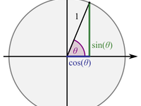
三角函数，正弦和余弦，有一个相对容易的计算方法：Taylor 展开。 我们都知道正弦函数有以下 Taylor 展开：

sin⁡x=∑n=0∞(−1)nx2n+1(2n+1)!=x−x33!+x55!−...\begin{aligned} \sin x &= \sum_{n=0}^\infty (-1)^n \frac{x^{2n+1}}{(2n+1)!} \\ &= x - \frac{x^3}{3!} + \frac{x^5}{5!} - ... \end{aligned}sinx​=n=0∑∞​(−1)n(2n+1)!x2n+1​=x−3!x3​+5!x5​−...​

我们可以观察到，每个展开项都可以用基本的算术运算来计算。 因此，我们可以在 Nix 中实现以下函数：

{
 pi = 3.14159265358979323846264338327950288;
 # Helper functions to sum/multiply all items in the array
 sum = builtins.foldl' builtins.add 0;
 multiply = builtins.foldl' builtins.mul 1;
 # Modulos function, "a mod b". Used for limiting input to sin/cos to (-2pi, 2pi)
 mod = a: b:
  if a < 0
  then mod (b - mod (0 - a) b) b
  else a - b * (div a b);
 # Power function, calculates "x^times", where "times" is an integer
 pow = x: times: multiply (lib.replicate times x);
 # Sine function
 sin = x: let
  # Convert x to floating point to avoid integer arithmetrics.
  # Also modulos it by 2pi to limit input range and avoid precision loss
  x' = mod (1.0 * x) (2 * pi);
  # Calculate i-th item in the expansion, i starts from 1
  step = i: (pow (0 - 1) (i - 1)) * multiply (lib.genList (j: x' / (j + 1)) (i * 2 - 1));
  # Note: this lib.genList call is equal to for (j = 0; j < i*2-1; j++)
 in
  # TODO: Not completed yet!
  0;
}

对于单个 Taylor 展开项的计算，为了避免精度损失，我没有在除法之前分别计算分子和分母。 相反，我将 xnn!\frac{x^n}{n!}n!xn​ 展开为 x1⋅x2⋅...⋅xn\frac{x}{1} \cdot \frac{x}{2} \cdot ... \cdot \frac{x}{n}1x​⋅2x​⋅...⋅nx​，并逐个计算它们，然后将所有这些较小的结果相乘。

然后，我们需要确定要计算多少项。 我们可以选择固定数量的项，例如 10：

{
 sin = x: let
  x' = mod (1.0 * x) (2 * pi);
  step = i: (pow (0 - 1) (i - 1)) * multiply (lib.genList (j: x' / (j + 1)) (i * 2 - 1));
 in
  # Invert when x < 0 to reduce input range
  if x < 0
  then -sin (0 - x)
  # Calculate 10 Taylor expansion items and add them up
  else sum (lib.genList (i: step (i + 1)) 10);
}

但是，当使用固定数量的项时，当输入非常小时，10 个 Taylor 展开项会迅速降低到浮点精度以下，而对于较大的输入，进一步的项仍然不够小，无法忽略。 所以我决定让它根据 Taylor 展开项的值做出决定，并在该值低于我们的精度目标时停止计算：

{
 # Accuracy target, stop iterating when Taylor expansion item is below this
 epsilon = pow (0.1) 10;
 # Absolute value function "abs" and its alias "fabs"
 abs = x:
  if x < 0
  then 0 - x
  else x;
 fabs = abs;
 sin = x: let
  x' = mod (1.0 * x) (2 * pi);
  step = i: (pow (0 - 1) (i - 1)) * multiply (lib.genList (j: x' / (j + 1)) (i * 2 - 1));
  # Stop if absolute value of current item is below epsilon, continue otherwise
  # "tmp" is the accumulator, and "i" is the index for the Taylor expansion item
  helper = tmp: i: let
   value = step i;
  in
   if (fabs value) < epsilon
   then tmp
   else helper (tmp + value) (i + 1);
 in
  if x < 0
  then -sin (0 - x)
  # Accumulate from 0, index start from 1
  else helper 0 1;
}

现在我们有了一个具有足够精度的正弦函数。 使用从 0 到 10（大于 2π2 \pi2π）的输入扫描其结果，步长为 0.001：

{
 # arange: generate an array from "min" (inclusive) to "max" (exclusive) every "step"
 arange = min: max: step: let
  count = floor ((max - min) / step);
 in
  lib.genList (i: min + step * i) count;
 # arange: generate an array from "min" (inclusive) to "max" (inclusive) every "step"
 arange2 = min: max: step: arange min (max + step) step;
 # Test function: calculate each value from array "inputs" with "fn", and generate an attrset for input -> output
 testOnInputs = inputs: fn:
  builtins.listToAttrs (builtins.map (v: {
    name = builtins.toString v;
    value = fn v;
   })
   inputs);
 # Test function: try all inputs from "min" (inclusive) to "max" (inclusive) every "step"
 testRange = min: max: step: testOnInputs (math.arange2 min max step);
 testOutput = testRange (0 - 10) 10 0.001 math.sin;
}

将 testOutput 与 Python Numpy 的 np.sin 的结果进行比较，所有结果都在真值的 0.0001% 以内。 这满足了我们的精度要求。

类似地，我们可以实现余弦函数：

{
 # Convert cosine to sine
 cos = x: sin (0.5 * pi - x);
}

你真的认为我要从头再做一遍吗？ 真的吗？

类似地，正切函数也很简单：

{
 tan = x: (sin x) / (cos x);
}

我还对 cos 和 tan 进行了测试，误差也在 0.0001% 以内。

arctan: 近似，唯一的方法

反正切函数也有一个 Taylor 展开：

arctan⁡x=∑n=0∞(−1)nx2n+12n+1=x−x33+x55−...\begin{aligned} \arctan x &= \sum_{n=0}^\infty (-1)^n \frac{x^{2n+1}}{2n+1} \\ &= x - \frac{x^3}{3} + \frac{x^5}{5} - ... \end{aligned}arctanx​=n=0∑∞​(−1)n2n+1x2n+1​=x−3x3​+5x5​−...​

然而，很容易注意到 arctan 的 Taylor 展开的收敛速度远不如正弦函数。 由于其分母线性增加，我们需要计算更多的项，直到它小于 epsilon，这可能会导致 Nix 的堆栈溢出：

error: stack overflow (possible infinite recursion)

那么，Taylor 展开不再是一种选择，我们需要一些计算速度更快的东西。 受 https://stackoverflow.com/a/42542593 的启发，我决定用多项式回归拟合 [0,1][0, 1][0,1] 上的反正切曲线，并使用以下规则映射其他范围内的反正切函数：

x<0,arctan⁡(x)=−arctan⁡(−x)x>1,arctan⁡(x)=π2−arctan⁡(1x)\begin{aligned} x < 0,& \arctan (x) = -\arctan (-x) \\ x > 1,& \arctan (x) = \frac{\pi}{2} - \arctan (\frac{1}{x}) \\ \end{aligned}x<0,x>1,​arctan(x)=−arctan(−x)arctan(x)=2π​−arctan(x1​)​

启动 Python 和 Numpy，开始拟合过程：

import numpy as np
# Generate input to arctan, 1000 points on [0, 1]:
a = np.linspace(0, 1, 1000)
# Polynomial regression, I'm using 10th order polynomial (x^10)
fit = np.polyfit(a, np.arctan(a), 10)
# Output regression results
print('\n'.join(["{0:.7f}".format(i) for i in (fit[::-1])]))
# 0.0000000
# 0.9999991
# 0.0000361
# -0.3339481
# 0.0056166
# 0.1692346
# 0.1067547
# -0.3812212
# 0.3314050
# -0.1347016
# 0.0222228

上面的输出意味着 [0,1][0, 1][0,1] 上的反正切函数可以用以下公式近似：

arctan⁡(x)=0+0.9999991x+0.0000361x2−...+0.0222228x10\arctan(x) = 0 + 0.9999991 x + 0.0000361 x^2 - ... + 0.0222228 x^{10}arctan(x)=0+0.9999991x+0.0000361x2−...+0.0222228x10

我们可以在 Nix 中复制这个多项式函数：

{
 # Polynomial calculation, x^0*poly[0] + x^1*poly[1] + ... + x^n*poly[n]
 polynomial = x: poly: let
  step = i: (pow x i) * (builtins.elemAt poly i);
 in
  sum (lib.genList step (builtins.length poly));
 # Arctangent function
 atan = x: let
  poly = [
   0.0000000
   0.9999991
   0.0000366
   (0 - 0.3339528)
   0.0056430
   0.1691462
   0.1069422
   (0 - 0.3814731)
   0.3316130
   (0 - 0.1347978)
   0.0222419
  ];
 in
  # Mapping when x < 0
  if x < 0
  then -atan (0 - x)
  # Mapping when x > 1
  else if x > 1
  then pi / 2 - atan (1 / x)
  # Polynomial calculation when 0 <= x <= 1
  else polynomial x poly;
}

我运行了精度测试，所有结果都在真值的 0.0001% 以内。

sqrt: 牛顿迭代法

对于平方根函数，我们可以使用著名的牛顿迭代法进行迭代。 我使用的迭代公式是：

an+1=an+xan2a_{n+1} = \frac{a_n + \frac{x}{a_n}}{2}an+1​=2an​+an​x​​

其中 xxx 是平方根函数的输入。

我们可以用以下代码在 Nix 中实现牛顿平方根计算，并迭代直到结果的变化低于 epsilon：

{
 # Square root function
 sqrt = x: let
  helper = tmp: let
   value = (tmp + 1.0 * x / tmp) / 2;
  in
   if (fabs (value - tmp)) < epsilon
   then value
   else helper value;
 in
  if x < epsilon
  then 0
  else helper (1.0 * x);
}

精度测试显示，所有结果都在真值的 1e−101e-101e−10（绝对值）以内。

Haversine 公式

有了上面的函数，我们终于可以开始实现 Haversine 公式了。 我使用来自 Stackoverflow 的这个实现作为参考：https://stackoverflow.com/a/27943

{
 # Convert degree to radian
 deg2rad = x: x * pi / 180;
 # Haversine formula, input a pair of latitudes/longitudes, output surface distance on Earth
 haversine = lat1: lon1: lat2: lon2: let
  # Treat the Earth as a sphere with radius of 6371km
  radius = 6371000;
  # Radian of latitude difference
  rad_lat = deg2rad ((1.0 * lat2) - (1.0 * lat1));
  # Radian of longitude difference
  rad_lon = deg2rad ((1.0 * lon2) - (1.0 * lon1));
  # Calculate based on formula
  a = (sin (rad_lat / 2)) * (sin (rad_lat / 2)) + (cos (deg2rad (1.0 * lat1))) * (cos (deg2rad (1.0 * lat2))) * (sin (rad_lon / 2)) * (sin (rad_lon / 2));
  c = 2 * atan ((sqrt a) / (sqrt (1 - a)));
 in
  radius * c;
}

最后，根据光速计算理论延迟：

{
 # 150000: distance light travels each millisecond, divided by 2 (for round trip)
 rttMs = lat1: lon1: lat2: lon2: floor ((haversine lat1 lon1 lat2 lon2) / 150000);
}

结论

我终于达到了我想要的目标：根据光速计算我的节点之间的理论网络延迟。

所有这些三角函数（和一些额外的数学函数）都可以从我的 GitHub 获取：https://github.com/xddxdd/nix-math

如果您正在使用 Nix Flake，您可以按如下方式使用该函数：

{
 inputs = {
  nix-math.url = "github:xddxdd/nix-math";
 };
 outputs = inputs: let
  math = inputs.nix-math.lib.math;
 in{
  value = math.sin (math.deg2rad 45);
 };
}