在 JAX 中使用 SDFs 和快速扫描算法
导航菜单
在 JAX 中使用 SDFs 和 Fast Sweeping 算法
- 2025年5月4日
- jax,
- simulation
这将会是一篇有趣的博客 - 我们将探索水平集背后的直觉、Eikonal 方程,并用 JAX 实现一个用于求解此方程的快速算法,称为快速扫描方法 (fast sweeping method)。
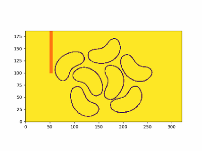 图 1: FSM 实际运行效果
我最近在研究一个问题,该问题涉及界面随时间的演变。我们的界面由一组点表示。为了使这个界面沿着其法线方向演变,我们近似计算这些点的法线,沿着法线方向延伸这些点,然后重新采样这些点以保持点密度——因为如果形状扩大了,点密度就会降低。这种传播界面的方法,涉及跟踪前沿上的粒子随其演变,被称为 Lagrangian front evolution,并伴随着一系列问题,例如重采样问题、处理“增长到”表面中的粒子等。
水平集方法和 Eikonal 方程 #
Sethian 和 Osher 提供了另一种传播界面的观点,他们发展了传播界面的水平集理论。关键区别在于这是一种 Eulerian 方法——界面是在固定的网格上隐式跟踪的,而不是像以前那样作为表面上的粒子。在水平集技术中,这种表面的隐式表示是一个函数的零水平集。这意味着,您将在网格上定义一个函数,并且该函数为零的网格点将代表您的表面。这个函数(我们称之为 ϕ\phiϕ)是水平集函数,并且是更高阶的函数,其输入为 x,y(在 2D 中)和_时间_。 ϕ(xgrid,ygrid,t=k)\phi(x_{grid}, y_{grid}, t=k)ϕ(xgrid,ygrid,t=k) 给出您在时间 kkk 的零水平集,描述您的界面。我们想要学习/近似的就是这个函数。在大多数时候,特定时间点的水平集函数是 signed distance function。
由水平集理论定义的初值问题允许沿法线方向的正向和负向传播速度。事实上,对于大多数涉及水平集技术的复杂问题,设计适当的传播速度至关重要,正如 Sethian 的书 中提到的那样。在本博客中,我们将考虑一种更简单的情况,即传播速度仅为正——这在几个重要的应用中都是如此。
我们将要寻找解的方程被称为 Eikonal 方程,它看起来像这样:
∣∇T∣F=1|\nabla T| F=1 ∣∇T∣F=1
这是一个双曲 PDE。如果您想象光从火焰中的某个点传播开来,那么 TTT 是火焰到达特定网格点的时间。 FFF 是传播速度,∇\nabla∇ 是梯度算子。 TTT 和 FFF 都是接受空间向量 xxx 作为输入的函数。您可以想象这在模拟波前时非常有用——例如,在 Huygens principle 中,新波上的每个点都充当次级小波的源,而波前是这些小波外部部分的包络。它也用于 seismic studies——因为波传播直接转化为这些,以及 shortest path 问题,medical imaging 等等。最近,它也被用于 construct signed distance functions (SDFs) of arbitrary geometry,这种表示方法越来越多地用于机器学习中 3D 表面的隐式表示。对于 SDFs, F=1F=1F=1。
Eikonal 方程可能会产生冲击和奇异性,例如,在障碍物附近或自塌陷曲线附近(参见图 2)。用于求解 Eikonal 方程的传统数值方法(将 PDE 离散化为在网格上定义的 ODE 系统,使用 Runge-Kutta 等数值积分器求解 ODE 等)不能很好地处理冲击和奇异性。例如,在存在障碍物的情况下,用于求解该方程的经典数值例程不会给您一个 signed distance function。因此,我们可以使用其他更高效的手工算法。
, showing how starting from a cosine front (bottom curve), propagating inward can result in a singularity (sharp point on the front). Also as you can see, markdown doeesnt render here.](https://rohangautam.github.io/img/dAfwLCSUSD-400.webp) 图 2:来自 Sethian 的论文 的图片,显示了从余弦波前(底部曲线)开始,向内传播如何导致奇异性(波前上的尖锐点)。
图 2:来自 Sethian 的论文 的图片,显示了从余弦波前(底部曲线)开始,向内传播如何导致奇异性(波前上的尖锐点)。
Fast sweeping 方法 #
Fast Marching Method (FMM),由 Sethian 引入,使用堆结构以 O(nlogn)O(n\log n)O(nlogn) 的时间复杂度(nnn 是网格大小)求解 Eikonal 方程,用于高效的最小值/最大值查询。Fast Sweeping Method (FSM),后来由 Hongkai Zhao 于 2005 年引入,以 O(n)O(n)O(n) 的时间复杂度完成此操作。这就是我们将要研究的。我们将考虑 2D 示例,尽管此算法可以推广到 n-D。
FSM 在扫描中执行计算 - 并且每个扫描都近似于沿一个方向的到达时间,并且这些扫描是隐式组合的,因为扫描是一个接一个发生的。在 2D 域中有 22=42^2=422=4 个方向。您可以在图 1 的动画中看到它的实际效果,其中有一些豆形初始波前和一个障碍物。
现在您已经有了一些直觉,让我们了解一下该算法的组成部分。
- 网格设置:与任何 Eulerian 近似一样,您将域划分为网格,并选择网格间距。您确定要从中开始传播的网格单元(源单元)以及路径中的任何障碍物。请注意,由于这些单元格被标记为“冻结” - 它们不参与计算。该算法基本上跳过了这些点。
- 您将源点的到达时间初始化为 0 - 这将是固定的。所有其他点都初始化为“足够大的值”[1]
- 在每次扫描中,您根据相邻单元格的值更新当前单元格的到达时间。在这里,我们局部求解 Eikonal 方程。空间导数由 Godunov 上风差分格式近似,该格式对 direction of information flow 敏感,这在此问题中至关重要。基本上,如果“波”从底部到达,例如,它应该主要使用来自这些单元格的值。您可以在 这里 阅读有关它的更多信息。这听起来像是一个花哨的术语,但事实并非如此,并且实现起来非常简单。局部求解 Eikonal 方程涉及求解二次方程(Zhao 的论文 中的方程 2.4)。
- 扫描覆盖坐标方向的 2n2^n2n(2D 中为 4)组合,确保从所有相对“象限”(例如,x 增加/y 增加,x 减小/y 增加等)传播的信息被上风格式正确捕获。如前所述,上风格式需要尊重信息流的方向,并且 4 次扫描中的每一次都从特定方向贡献信息,所有这些信息都组合在最终算法中。
代码 #
我可以谈论的就这么多了。要真正理解它,请玩玩代码。我将首先向您展示 numpy 代码,这更容易理解,然后再转到 JAX 代码。JAX 代码的逻辑相同,但为了提高效率,事情使用即时编译重新组织。我喜欢这些算法的原因是,由于界面传播是一个如此直观的问题,因此看到它们的输出并使用代码可能会非常吸引人。所有代码都可以在 这个 repo 中找到,并且您会发现 this demo notebook 是一个开始使用的好地方 [2]。
numpy #
import numpy as np

def fast_sweep_2d(grid, fixed_cells, obstacle, f, dh, iterations=5):
  # this is used for padding the outer boundaries of the domain,
  # so that the min() operations in the upwind scheme choose the inner point.
  large_val = 1e3
  nx, ny = grid.shape
  # 4 directions to sweep along - the range parameters for x and y.
  sweep_dirs = [
    (0, nx, 1, 0, ny, 1), # Top-left to bottom-right
    (nx - 1, -1, -1, 0, ny, 1), # Top-right to bottom-left
    (nx - 1, -1, -1, ny - 1, -1, -1), # Bottom-right to top-left
    (0, nx, 1, ny - 1, -1, -1), # Bottom-left to top-right
  ]
  # pad with a large value to properly handle boundary conditions in the upwind scheme.
  padded = np.pad(grid, pad_width=1, mode="constant", constant_values=large_val)
  for _ in range(iterations):
    for x_start, x_end, x_step, y_start, y_end, y_step in sweep_dirs:
      for iy in range(y_start, y_end, y_step):
        for ix in range(x_start, x_end, x_step):
          # dont do anything for fixed cells (interface) or obstacles
          if fixed_cells[iy, ix] or obstacle[iy, ix]:
            continue
          # calculate a,b from eqn 2.3 of Zhao et.al
          py, px = iy + 1, ix + 1
          # since it's a padded array and boundary+1 is a large value,
          # it will choose the interior value at the end, acting like one sided difference.
          a = np.min((padded[py, px - 1], padded[py, px + 1]))
          b = np.min((padded[py - 1, px], padded[py + 1, px]))
          # explicit unique solution to eq 2.3, given by eq 2.4
          xbar = (
            large_val # xbar will be the distance to this cell from front
          )
          if np.abs(a - b) >= f * dh:
            xbar = np.min((a, b)) + f * dh
          else:
            # can add small eps to sqrt later for stability
            xbar = (a + b + np.sqrt(2 * (f * dh) ** 2 - (a - b) ** 2)) / 2
          # update if new distance is smaller
          padded[py, px] = np.min((padded[py, px], xbar))
  # return un-padded array
  return padded[1:-1, 1:-1]
您可以这样调用它:
out = fast_sweep_2d(
  dist_grid_np, # initial distance grid - 0 at interface, large val everywhere else
  interface_mask, # 1 at interface, 0 elsewhere
  obstacle_mask,
  f=1, # propagation speed
  dh=dh, # grid spacing - is 1 for an image
  iterations=5,
)
jax #
这是 JAX 中的代码!
import jax
import jax.numpy as jnp
from functools import partial

@partial(jax.jit, static_argnames=["iterations"])
def fast_sweep_2d(grid, fixed_cells, obstacle, f, dh, iterations=5):
  large_val = 1e3
  nx, ny = grid.shape
  sweep_dirs = [
    (0, nx, 1, 0, ny, 1), # Top-left to bottom-right
    (nx - 1, -1, -1, 0, ny, 1), # Top-right to bottom-left
    (nx - 1, -1, -1, ny - 1, -1, -1), # Bottom-right to top-left
    (0, nx, 1, ny - 1, -1, -1), # Bottom-left to top-right
  ]
  frozen = jnp.logical_or(fixed_cells, obstacle)
  padded = jnp.pad(grid, pad_width=1, mode="constant", constant_values=large_val)
  def run_sweep(sweep_dir, grid):
    x_start, x_end, x_step, y_start, y_end, y_step = sweep_dir
    def y_loop_body(iy, grid):
      def x_loop_body(ix, grid):
        piy, pix = iy + 1, ix + 1
        a = jnp.minimum(grid[piy, pix - 1], grid[piy, pix + 1])
        b = jnp.minimum(grid[piy - 1, pix], grid[piy + 1, pix])
        updated_val = jnp.where(
          frozen[iy, ix],
          grid[piy, pix], # no change if frozen
          jnp.minimum( # min of curr and updated val
            grid[piy, pix],
            jnp.where( # eqn 2.4
              jnp.abs(a - b) >= f * dh,
              jnp.minimum(a, b) + f * dh,
              (a + b + jnp.sqrt(2 * (f * dh) ** 2 - (a - b) ** 2)) / 2,
            ),
          ),
        )
        return grid.at[piy, pix].set(updated_val)
      x_indices = jnp.arange(x_start, x_end, x_step)
      return jax.lax.fori_loop(
        0,
        len(x_indices),
        # ix is 0..len(x_indices) - we need to map it to actual range
        lambda ix, grid: x_loop_body(x_indices[ix], grid),
        grid,
      )
    y_indices = jnp.arange(y_start, y_end, y_step)
    return jax.lax.fori_loop(
      0,
      len(y_indices),
      lambda iy, grid: y_loop_body(y_indices[iy], grid),
      grid,
    )
  def iteration_body(_, cur_grid):
    # perform 4 sweeps (2 dimentions)
    grid_s1 = run_sweep(sweep_dirs[0], cur_grid)
    grid_s2 = run_sweep(sweep_dirs[1], grid_s1)
    grid_s3 = run_sweep(sweep_dirs[2], grid_s2)
    grid_s4 = run_sweep(sweep_dirs[3], grid_s3)
    return grid_s4
  final_grid = jax.lax.fori_loop(0, iterations, iteration_body, padded)
  return final_grid[1:-1, 1:-1]
实际应用 #
这是一个 Fast sweeping 方法的实际应用示例。我们有一些豆形轮廓(在 这里 制作,呵呵),我将其处理为边界处为(灰度)0,其他地方为 255。我还添加了一个障碍物(红色)。我们可以看到它计算距离函数(不是_signed_ distance function),方法是注意 t=5t=5t=5 的豆子内部的轮廓。如果您想要一个 SDF,则需要提供符号信息。例如,如果我们有一个与网格形状相同的矩阵,形状内部为 -1,表面为 0,外部为 1,我们可以简单地将此矩阵与距离函数相乘,以获得 signed distance function。我提到 SDFs,因为使用 FSM 生成 SDFs 很常见。在这种情况下,我没有计算符号信息,所以我在下面只留下距离场。我们使用等高线来可视化不同时间点的波前。
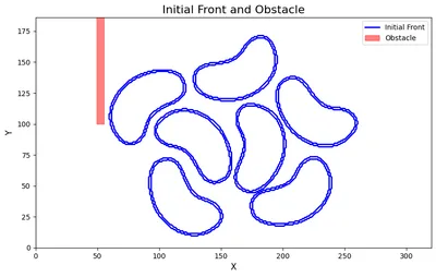 图 3:初始设置
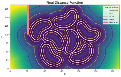 图 4:计算出的距离场,带有采样到达时间的轮廓。有关 FSM 的实际应用,请参见图 3。
基准测试 #
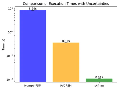
我在我的 Apple M2 Pro 芯片上运行了一些基准测试。我们可以看到,正如预期的那样,在 CPU 上编译的 JAX 代码比 numpy 代码快得多。请注意此图 y 轴上使用的对数刻度。我还将其与 FMM 库——skfmm 进行了比较。库中的逻辑是用 C++ 编写的,因此比此处讨论的两种方法都更快。但是,当使用自定义 FSM 方法解决特定领域问题时,我宁愿用 python 代码获得的易于 hack 和实验的特性来换取 skfmm 的速度。当然,您可能会很乐意 hack C++ 代码 :)
关于并行 FSM 的说明 #
实际上,我尝试通过并行化该算法来进一步加快速度,如 Hongkai Zhao 的后续论文 的 2.1 节中所述。还有其他 more complex parallel FSM implementations,但我现在没有研究它们。Zhao 的后续论文中的想法是并行运行扫描,然后使用元素最小值运算将它们全部组合起来。这似乎是一个足够简单的改变,但_专门使用 JAX_,我无法找到一种方法来做到这一点。挑战是一个经典的 JAX 问题——定义计算形状的变量无法被跟踪。我试图在扫描方向上进行 vmap,但由于它们构成了 arange 函数的参数,该函数确定了计算形状,因此我无法让这些成为跟踪值——并且 by definition vmap works with tracing 它的输入数据。任何类型的数据/变量重组都无法实现这一点。致读者——如果有一种解决此问题的技巧,我很乐意知道!!
参考资料 #
-
Level Set Methods and Fast Marching Methods : Evolving Interfaces in Computational Geometry, Fluid Mechanics, Computer Vision, and Materials Science
-
以及本博客上的其他超链接 :D
-
我使用
1e3。 ↩︎ -
该笔记本电脑还包含本博客中所有视觉效果的代码! ↩︎