27000条龙和10000盏灯：GPU驱动的Clustered Forward渲染器

27000 Dragons and 10'000 Lights: GPU-Driven Clustered Forward Renderer

Source | HN Comments

文章介绍了一个基于 GPU-Driven 的 Clustered Forward 渲染器，该渲染器能够在 GTX 1070 上以超过 60fps 的速度渲染 27000 个模型和 10000 盏灯。文章详细阐述了 GPU-Driven 渲染的优势，包括减少 draw call、使用 compute shader 进行剔除和压缩 draw buffer。此外，文章还介绍了 Clustered Shading 技术，通过将视锥体分割成集群来减少片段着色成本，并给出了集群分配和着色实现的细节。最后，文章展示了渲染器的性能结果，并分享了代码和优化策略。

logdahl.net / 27'000 dragons and 10'000 lights: GPU-Driven Clustered Forward Renderer

2025/04/15 在 Advanced Computer Graphics and Applications 课程中，我有大量的时间（和自由！）来开发一些有趣的东西。虽然这是一篇关于计算机图形学的文章，但它也关于高性能并行化策略。我编写了一个使用 clustered shading 的 GPU-Driven forward 渲染器。它可以在 GTX 1070 GPU 上以超过 60fps 的速度渲染 27'000 个 stanford dragons 和 10'000 盏灯，分辨率为 1080p。在这篇文章中，我将详细介绍我的渲染器是如何实现这种性能的。 <RawText children='dragons.'> dragons.

什么是 GPU-Driven？

在传统的渲染器中，GPU 和 CPU 在内存和所有权方面存在某种分离。通常，GPU 拥有纹理数据、网格和其他资源，而 CPU 拥有实体数据（位置、速度等）。这通常是一个好的设计，因为实体数据在 CPU 上被多次修改，并且每帧通过 uniform 或类似的方式上传一次到 GPU。然而，这意味着需要在编写每个对象的数据和渲染它之间设置一些障碍。重要的是，为所有对象使用单个 uniform 需要按顺序在各自的 draw call 中渲染每个对象。我们的目标是尽可能减少 draw call 的数量。在 GL 和 Vulkan 中，都存在一个用于 indirect multi draws 的 API。这些 API 与普通的 draw call 不同，CPU 在缓冲区中已存在的 draw 细节（索引计数、起始顶点索引）的情况下调度指令。这样，一个 API 调用可以执行多个 draw call。这导致了一些限制——例如，在 draw call 之间重新绑定资源或更改 shader 是不可能的——但这是为了性能而做出的权衡。在我的渲染器中，实体（对象）数据保存在一个连续的缓冲区中，并且任何对其进行的修改都会被标记。在渲染一帧之前，所有修改的部分都会被上传到 GPU。

内存

Vertex Buffer Index Buffer Material Buffer Object Buffer Material ID Transform Draw Buffer Vk Indexed Draw Indirect Command Object Index Count Instance Count First Index Vertex Offset First Instance 1 Mesh Buffer Start Index Index Count distance Start Index Index Count distance LOD 0 LOD 1 Mesh ID Bounding Box 用于驱动渲染的 GPU 缓冲区。在上图中，显示了选择的 GPU 缓冲区。与其他一些渲染器一样，我们为所有顶点数据共享一个 GPU 缓冲区。相反，我们使用一个简单的分配器来自动管理这个连续的缓冲区。这也适用于索引缓冲区。这样做有一个缺点：它要求所有顶点具有相同的格式（相同的属性）。如果场景中有许多不同类型的网格，这可能会成为一个问题。一种解决方案是为某些属性使用单独的顶点缓冲区，这也可以提高缓存一致性，从而提高性能。例如，可能需要为动画顶点创建一个单独的缓冲区，或者仅为动画属性（骨骼 ID、权重等）创建一个单独的缓冲区。我们还有一些这个系统独有的缓冲区；即 Object Buffer 和 Draw Buffer。这些包含传统 CPU 驱动的渲染器必须每帧提供给 GPU 的信息，但这些信息改为存储在设备上。完全静态的对象（例如地形）只需要上传一次。 draw buffer 实际上减少了 CPU draw call 的数量（使用前面提到的 draw indirect API）。

Draw Call 生成

对于优化的渲染器，我们希望剔除主摄像机视锥体之外的对象。从缓冲区图中可以看出，我们实际上拥有确定需要渲染的内容所需的一切（除了摄像机）。由于我们现在从 GPU 创建 draw call（到 Draw Buffer 中），因此 GPU 现在能够剔除场景，这应该会带来显着的加速。我通过让网格存储一个轴对齐的边界框（AABB）来简化了这一点。虽然可以使用其他形状（只需在前面加上一个标志），但这在我的情况下效果很好。 X X X Batch 0 Batch 1 Object Buffer Draw Buffer 从 GPU 上的 Object Buffer 到 Draw Buffer 的剔除。使用 compute shader，如果对象可见，则从每个对象创建 draw buffer 中的元素。一个简单的实现是插入到与原始对象定义所在的相同索引中。这意味着剔除可以非常并行化，其中子组的每个线程剔除单个对象。这种设计的一个缺点是，最终的 draw buffer 变得稀疏；因此需要比必要的更多的内存。如果我们假设有时所有对象都可见，这将是可以的，因为我们需要这么大的缓冲区。但通常，游戏可能会剔除多达 70% 或更多的对象数量。开发人员运行游戏并发现单个帧中显示的物体不超过全部物体的 50%，这意味着 draw buffer 可以小到物体缓冲区的 50%。此外，我们可以预期性能会得到提高（假设压缩很快），因为 draw 元素将改善空间局部性。另一个需要考虑的事情是，NOP draw indirect 调用（即具有 0 个顶点的调用）实际上并不是免费的，因此我们也可以预期 draw 会更快。在我的 GTX 1070 上运行，渲染 12.5 万个被剔除的物体需要 2.97 毫秒的开销（平均每个物体 23 纳秒）。需要特别注意支持多个 shader。虽然我不需要它，但我尝试实现它，但只遇到了问题。问题是必须为每个 shader 分配一个估计可以使用该 shader 绘制的对象数量。要么将两个 draw list 存储在同一个缓冲区中（为 shader A 保留 70%，为 shader B 保留 30%），要么创建 2 个不同的缓冲区。

压缩

为了支持这一点，我们希望压缩插入到 draw buffer 中的元素，以便它们连续存在。这实际上很容易使用原子计数器来实现。在每一帧的开始，计数器都会重置为零。对于每个需要渲染的对象，原子计数器都会递增。 Draw 被插入到原子计数器给定的索引上。简单，是的！性能好吗？马马虎虎。嗯，实际上也很容易优化它。 GPU 编程很有趣，因为与 SIMD 指令类似，最有效的用法来自于对协作的充分考虑。在这种情况下，我们将使用使用 ballots 的子组操作来加速集群压缩。 Ballots 只是一个位集，其中子组中的每个线程都拥有它。例如，每个线程可以评估一个布尔值，然后将其分配给位集中的槽。它还具有用于评估整个 ballot 的廉价操作，例如加法、位计数等。我发现这个算法很难解释，所以我在下面提供了我的代码和解释它的图表。 1 0 1 0 1 1 1 0 0 1 0 1 Subgroup Visibility Ballot 0 1 1 2 2 3 4 5 5 5 6 6 Prefix Sum Local Offset 7 7 7 7 7 7 7 7 7 7 7 7 Local Count Atomic Add Draw Count 2 Base Offset Broadcast 2 2 2 2 2 2 2 2 2 2 2 2 Draw List Index Base + Local 3 3 4 4 Draw Buffer 5 6 7 7 7 8 8 Broadcast Base Offset 用于优化 draw-list 压缩的 Ballot 操作。``` void main() { uint idx = gl_GlobalInvocationID.x; uint local_id = gl_LocalInvocationID.x; uint object_id = idx; uint mesh_id = objects[object_id].mesh_id; // Skip invalid objects (those with no geometry) if (mesh_id == -1) return; mat4 affine_transform = unpack_affine_transform(object_id); bool visible = is_visible(object_id, affine_transform); uvec4 valid_mask = subgroupBallot(visible); uint local_offset = subgroupBallotExclusiveBitCount(valid_mask); uint local_count = subgroupBallotBitCount(valid_mask); uint base_offset = 0; if (subgroupElect()) { base_offset = atomicAdd(draw_count, local_count); } base_offset = subgroupBroadcastFirst(base_offset); if (visible) { uint lod = get_lod(object_id, affine_transform); uint draw_idx = base_offset + local_offset; uint index_count = meshes[mesh_id].lods[lod].index_count; uint index_start = meshes[mesh_id].lods[lod].index_start; emitDraw(draw_idx, index_count, index_start, object_id); atomicAdd(stats.draw_count, 1); atomicAdd(stats.draw_count_lod[lod], 1); } }


在使用此算法后，绘制 12.5 万个剔除对象的开销缩小到 0.9 毫秒的 _静态_ 成本（作为单个空 draw indrect 调用）。
以下是一些测量结果，其中包含 27'000 个 Stanford dragons 的单个场景在 RTX A2000 12GB 上以 1080p 渲染。 总体而言，我们的指标显示：
  * 所有 dragons 都在一个批次中渲染
  * 大约 5'000 个实际上被绘制
  * 大约 5100 万个输入顶点和 1700 万个输入三角形
  * 3000 万个顶点调用
  * 根据方向，2-6 百万个片元调用


虽然与没有显示如何实现的“传统” CPU 渲染器进行比较似乎很奇怪，但这些测量结果应该非常典型，并且主要用于显示对比。
Dragons| CPU-Driven w/o Culling| GPU-Driven + Culling  
---|---|---  
CPU| Draw| CPU| Draw| Cull  
27'000| 2.9ms| 22.2ms| 120.1μs| 30.7μs| 9.3ms  
# Forward Clustered Shading
经典的 forward 渲染器存在一些问题，其中最大的问题通常是 overdraw。 overdraw 的片段既浪费工作，又浪费 GPU 填充率。 由于每个片段都以 forward 方式渲染，因此对于不可见的片段会发生昂贵的照明计算。 从历史上看，有人提出 deferred rendering 来解决这个问题。 通过仅渲染每个对象的 albedo、法线和其他属性，然后在像素上进行 shading，shading 仅在每个可见片段上执行。 虽然这解决了 overdraw 问题，但 deferred shading 带来了与带宽以及 anti-aliasing 相关的其他问题。
overdraw 问题可以通过多种方式处理，例如执行早期仅深度通道或通过三角形重新排序。 在这里，我专注于通过降低片段 shading 的成本来减轻 overdraw 的影响。 我们将使用所谓的 _Clustered Shading_ 来降低 shading 的成本。 在这种情况下，尝试一种先进技术并似乎非常适合我们已经概述的 GPU-Driven 结构都感觉很有趣。 我们已经是 bindless 的，并且已经将 lights 保留在 GPU 上，那么为什么不呢？
Clustered shading 是一种通过减少针对每个片段测试的光源数量来减少照明计算的方法。 该方法通过将视锥体分成称为集群（或 froxel）的视锥体形状的盒子，并根据其影响半径将光源分配给集群来工作。 在 shading 时，每个片段都可以查找包含的集群，并且仅使用这些光源计算 shading。 这意味着没有光源的集群不执行任何照明计算。
froxel 实际上是倾斜的视锥体，但在视图空间中将简化为 AABB。 虽然这是不正确的（一些片段最终出现在 2 个集群中！），但这使得相交计算更便宜，并且在现实中不是问题。
许多设计决策都受到 SIGGRAPH 上 Doom 讲座的启发（[Rendering The Hellscape Of Doom Eternal](https://logdahl.net/p/<https:/advances.realtimerendering.com/s2020/RenderingDoomEternal.pdf>) 和 [The Devil Is In The Details](https://logdahl.net/p/<https:/advances.realtimerendering.com/s2016/Siggraph2016_idTech6.pdf>））。 有趣的是，它们将集群方法重用于其他影响体积系统，例如贴花和 light probe。 我很想更深入地研究这个！
我们将为集群引入 3 个新缓冲区； _Cluster Buffer_ 、 _Cluster Items Buffer_ 和 _Light Buffer_。 light buffer 包含所有场景的点光源（或可以扩展到所有具有影响体积的光源）。 cluster buffer 包含实际的集群，这将是一个固定集。 cluster items buffer 用作集群引用光源的间接方式。
Light Buffer
Bounds Min
Bounds Max
Start
Hash & Num Lights
Position
Color
Falloff Linear, Quad
Cluster
0
2
3
9
Cluster Items
Clusters
5
Light
0
2
3
5
Start: 0
Hash: X
Num: 4
0
Start: 4
Hash: Y
Num: 1
1
Start: 5
Hash: X
Num: 4
2
用于集群的 GPU 缓冲区。
与对象缓冲区类似，light buffer 是 CPU 可访问的（写入来自 CPU），因此支持动态光源。
# 集群分配
将光源分配给集群是这个系统复杂的部分。 在此通道之后，每个集群都将引用集群项目的开始，以及哈希和光源数量。 每个集群最多支持 255 个光源。
分配是使用简单的 AABB 球体相交测试完成的。 由于光源不存储其半径，因此需要使用强度和衰减参数来计算。 一个简单的朴素实现类似于 Draw Buffer 剔除的工作方式。 让每个调用处理一个集群，然后直接遍历所有光源。 每个调用使用原子计数器保留一系列集群项目，最后写入索引。 使用这种朴素的方法，大约 10′000 个光源可以在 GTX 1070 上在 6 毫秒内分配给 2′800 个集群。 虽然这是一个极端情况，但仍有改进的空间。
此方法需要大量的内存访问（尽管它们大多是相干的），并且重复光源半径计算。 另一个问题是所需的内存量非常高，因为集群之间没有通信。 因此，每个集群都需要保留最坏情况下的内存量。 如果使用 16x8x24 网格，这将需要 3.1MB 的内存。 还要考虑到在 shading 期间查找项目时，items buffer 中会出现稀疏查找。
我们将再次应用压缩，并仔细考虑线程如何协作。 在此方法中，集群分配分为多个阶段； 预取、相交和写入。 这些阶段需要显式屏障，以确保所有调用都同步。 优化的方法使用光批次，批次大小与工作组的大小相同。 首先，每个调用协作地将以下批次的单个光源读入共享内存。 此后，已计算出所有光源的半径。 相交测试的工作方式与以前相同，仍然使用相干读取，但从共享内存中读取。 每个调用都保留一个相交光源 ID 的运行哈希，并将光源存储到调用私有内存中。 在没有更多批次要处理后，将比较调用哈希。 如果多个调用具有相同的哈希，则具有最低 ID 的调用会将来自私有内存的光源写入集群列表，并原子地递增列表中的项目数。 此实现如下所示。
Cluster 0
0
Cluster 1
Cluster bounds lookup
Light Prefetch
Invocation 0
Invocation 1
0
1
Count: 5
Hash: X
Count: 5
Hash: Y
Update Light Count & Hash
1
0
1
Light intersection
Cluster 2
2
Cluster 3
Invocation 2
Invocation 3
0
1
Count: 5
Hash: X
Count: 4
Hash: Z
3
0
1
2
2
2
2
3
3
3
3
4
5
4
4
4
4
5
5
5
5
0
1
0
2
Find First Same Hash
Range
0-5
Reserve range & Write
Range
5-10
Range
10-14
子组内协作策略的水平时间线。 6 个光源用于 4 个集群。
使用此方法，通过完全压缩，将 10'000 个光源分配给 2'800 个集群仅花费 1.1 毫秒，并且仅需要 164KB 的集群项目内存！
Naive| Collaborative| Full  
---|---|---  
Time| 6ms| 1.3ms| 1.1ms  
Memory| 3.1MB| 3.1MB| 164KB  
此方法可以进一步优化。 由于我们执行预通道，因此调用可以协作地将光源剔除到整个视锥体，从而减少所需的工作量。 虽然这尚未实现，但不应该太难。
以下是提供的 compute shader。 它真的很长而且有点令人困惑，但我认为它可能会帮助那些希望实现类似系统的人。 或者你知道，只是看看不同的并行化策略很有趣！

layout(local_size_x = 128) in; shared vec4 shared_lights[128]; shared uint shared_hashes[128]; shared uint shared_starts[128]; shared uint shared_first_invocation_with_hash[128]; void main() { uint cluster_index = gl_GlobalInvocationID.x; uint cluster_item_count = 0; uint cluster_item_offset = cluster_index * MAX_CLUSTER_ITEMS; vec3 cluster_min; vec3 cluster_max; uint private_items[MAX_CLUSTER_ITEMS]; if (cluster_index_valid(cluster_index, cluster_constants)) { cluster_min = clusters[cluster_index].bounds_min.xyz; cluster_max = clusters[cluster_index].bounds_max.xyz; } uint hash = hash_fnv1a_init(); uint local_index = gl_LocalInvocationID.x; for (uint batch_start = 0; batch_start <= highest_light; batch_start += 128) { uint light_batch_count = min(128, highest_light + 1 - batch_start); // Cooperatively cache this batch of lights and calculate their radii // Here we can also perform an early cull if the light is outside the frustum. barrier(); if (local_index < light_batch_count) { uint light_id = batch_start + local_index; LightData light = lights[light_id]; vec4 position_ws = light.position; vec3 position = vec3(push.view * position_ws); position *= -1; float intensity = distance(light.color.rgb, vec3(0.0)) * light.color.a; float radius = calculate_light_radius( light.falloff_linear, light.falloff_quadratic, intensity ); shared_lights[local_index] = vec4(position, radius); } barrier(); // Process this batch of lights if (cluster_index_valid(cluster_index, cluster_constants)) { for (uint i = 0; i < light_batch_count; i++) { if (cluster_item_count >= MAX_CLUSTER_ITEMS) break; uint light_id = batch_start + i; vec4 packed = shared_lights[i]; if (sphere_aabb_intersect(packed.xyz, packed.w, cluster_min, cluster_max)) { private_items[cluster_item_count] = light_id; cluster_item_count++; hash = hash_fnv1a_next(hash, light_id); } } } } hash = hash_fnv1a_next(hash, cluster_item_count); shared_hashes[local_index] = hash; shared_first_invocation_with_hash[local_index] = 0xFFFFFFFF; barrier(); if (!cluster_index_valid(cluster_index, cluster_constants)) return; // scan the subgroup for the first thread with the same hash as us for (uint i = 0; i < 128; i++) { if (i > local_index) continue; if (hash == shared_hashes[i]) { atomicMin(shared_first_invocation_with_hash[local_index], i); } } bool is_first = shared_first_invocation_with_hash[local_index] == local_index; uint first = shared_first_invocation_with_hash[local_index]; if (is_first) { uint start = atomicAdd(cluster_items_size, cluster_item_count); shared_starts[local_index] = start; for (uint i = 0; i < cluster_item_count; i++) { cluster_items[start + i] = private_items[i]; } } barrier(); clusters[cluster_index].item_start = shared_starts[first]; clusters[cluster_index].hash_and_num_lights = cluter_hash_and_count(hash, cluster_item_count); }


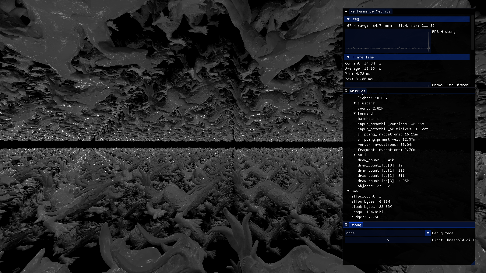
继续，看看图片！
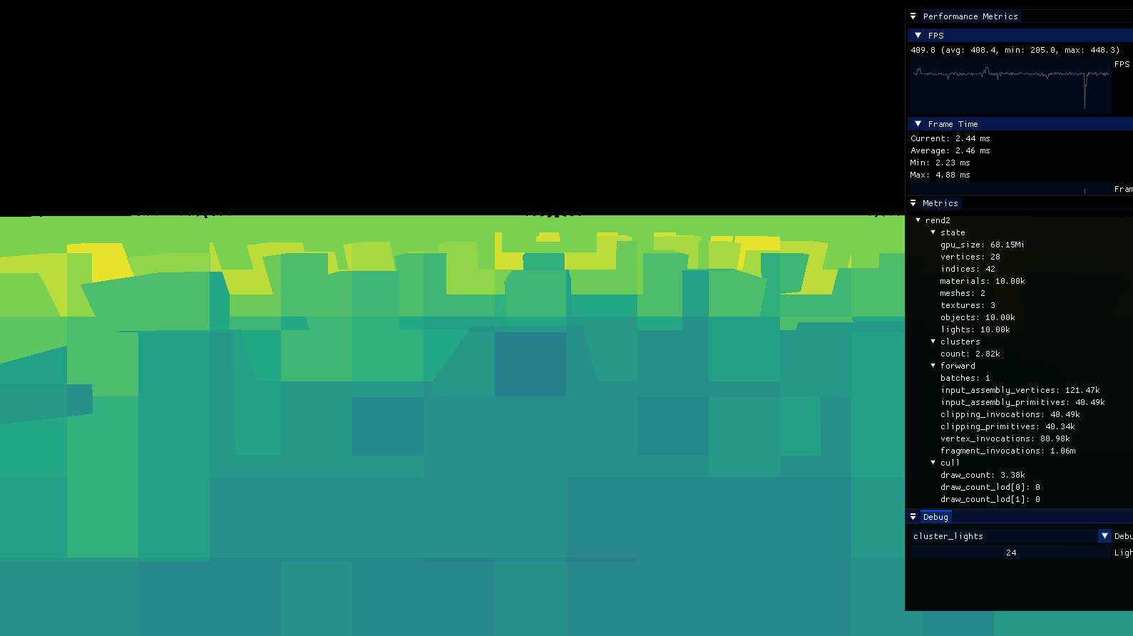![<RawText children='Number of lights per cluster.'>](https://logdahl.net/i/gpu-driven/cluster-count.png)每个集群的光源数量。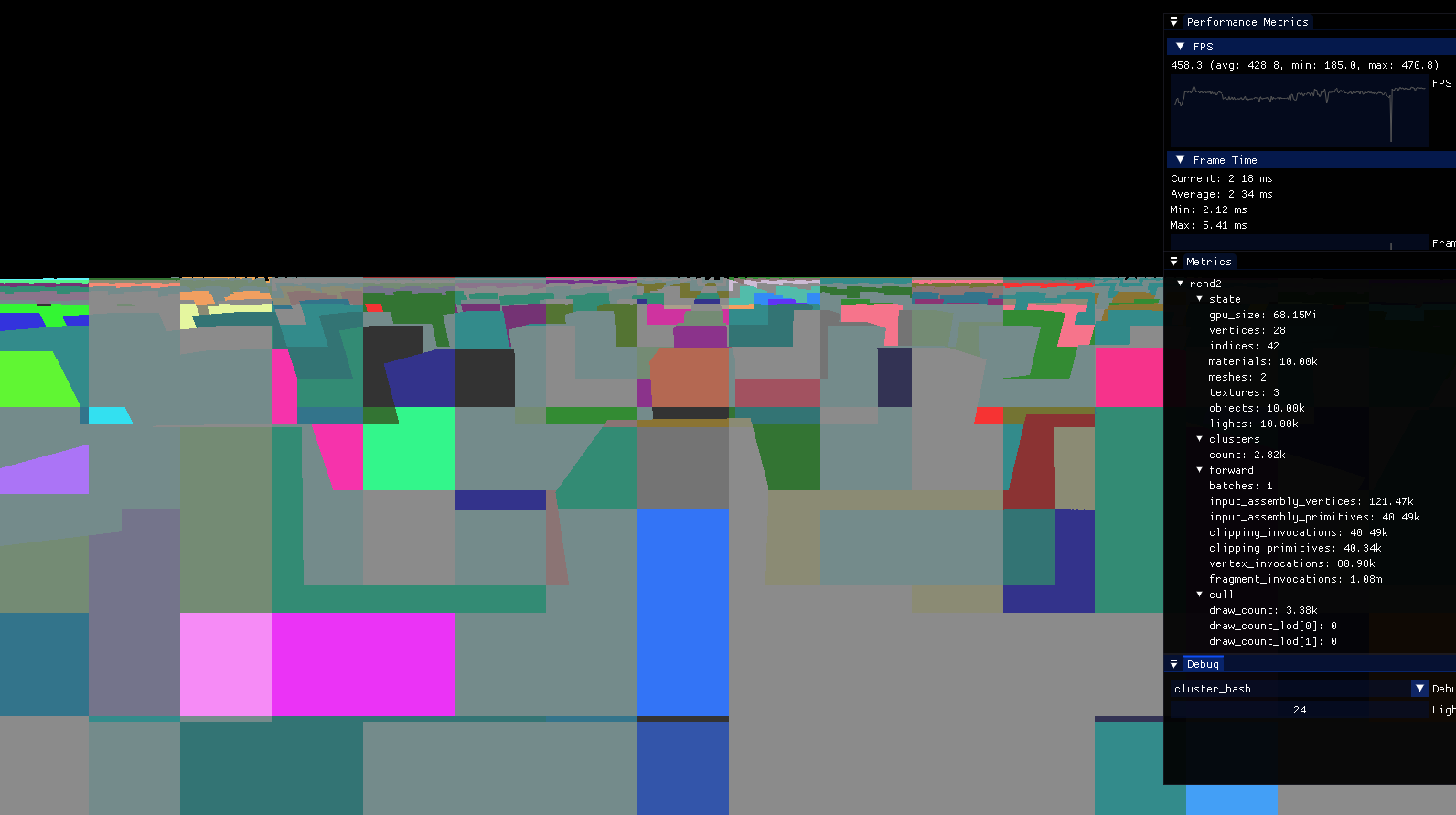![<RawText children='Overlay colored by the hash of each clusters.'>](https://logdahl.net/i/gpu-driven/cluster-hash.png)根据每个集群的哈希着色的覆盖。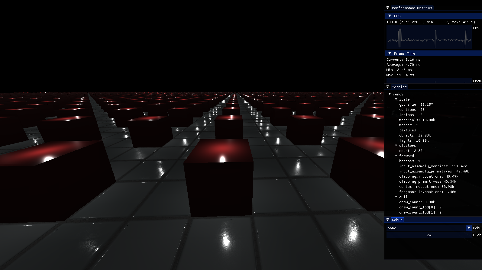![<RawText children='Colorized!'>](https://logdahl.net/i/gpu-driven/cluster-img.png)着色！
# 集群 Shading
最后，集群数据可用于 shading。 在 shading 给定片段时，我们计算给定视图空间片段位置的集群索引。 然后，我们可以遍历集群中的所有光源，并使用光源对片段进行 shading。
通常，同一子组中的多个片段将包含在同一集群中。 这意味着在理论上，我们应该能够通过在子组内共享信息来对此进行优化。 我的解决方案使用 ballots 来确定整个子组是否包含在相同的集群哈希中，如果是，则以标量方式读取光源。 这应该意味着，我们可以使内存访问更加相干，而不是执行矢量化读取并存储在 VGPR（矢量通用寄存器）中。 RDNA 架构具有专门的标量缓存和针对 VGPR 优化的操作，这意味着这应该更快。 但是，这对 NVIDIA GPU 具有负面性能影响。 它没有那么慢，但可能希望根据架构打开或关闭此功能。 也可能是我对这个的实现是错误的，但我无法在 RDNA 上测试它:)
标量读取在下图中显示为绿色。
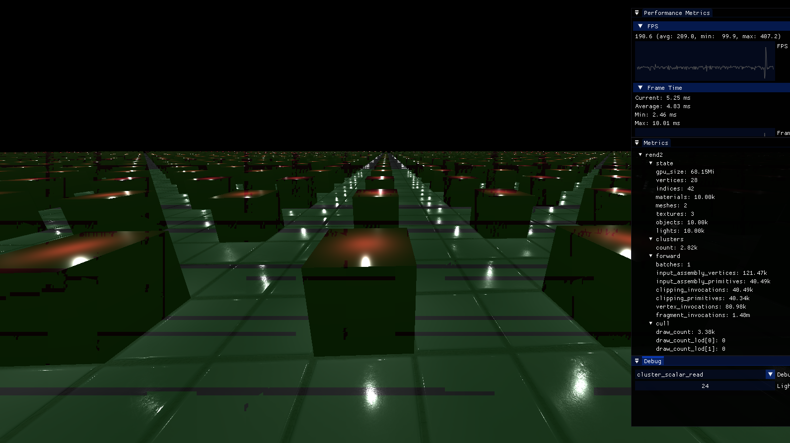![<RawText children='Overlay colored green if scalar read.'>](https://logdahl.net/i/gpu-driven/cluster-scalar.png)如果标量读取，则覆盖着绿色。
最后，片段 shader 看起来像这样：

void main() { ... uint cluster_id = cluster_lookup(position_vs, cluster_constants); uint cluster_hash; uint cluster_num_lights; cluster_unpack_hash_and_count(clusters[cluster_id].hash_and_num_lights, cluster_hash, cluster_num_lights); PbrProperties props = PbrProperties( albedo, roughness, metallic); // if entire subgroup in the same cluster, we can read only once bool subgroup_same_hash = subgroupAllEqual(cluster_hash); if (subgroup_same_hash) { uint group_cluster_id = subgroupBroadcastFirst(cluster_id); uint group_num_lights = subgroupBroadcastFirst(cluster_num_lights); uint first_cluster_item = clusters[group_cluster_id].item_start; uint last_cluster_item = first_cluster_item + group_num_lights; for (uint i = first_cluster_item; i < last_cluster_item; i++) { uint cluster_item = cluster_items[i]; uint light_id = cluster_item; LightData light = lights[light_id]; color += point_light_shade(P, N, V, light, props); } } else { for (uint i = 0; i < cluster_num_lights; i++) { uint cluster_item = cluster_items[clusters[cluster_id].item_start + i]; uint light_id = cluster_item; LightData light = lights[light_id]; color += point_light_shade(P, N, V, light, props); } } outColor = vec4(color, 1.0); }


# 结果
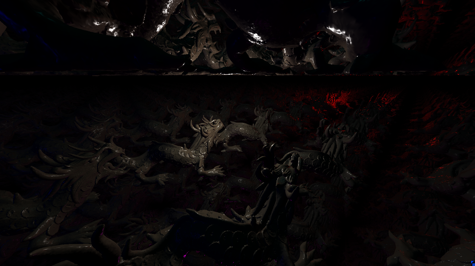
好吧，让我们诚实一点。 27'000 个 dragons 和 10'000 盏灯是可能的，但只是勉强可能。 它要求将光源的影响半径降低到其功率的 1/6。 在此场景中，它明显会导致伪影。 具体来说，当有许多光源密集堆积时，每个光源贡献 1% 仍然意味着它们一起贡献 10'000%！ 性能和所需的常量确实取决于场景。 这是一个不合理的场景。 在第二张图片中，你可以更好地看到动态范围（但遗憾的是看不到成千上万的 dragons）。
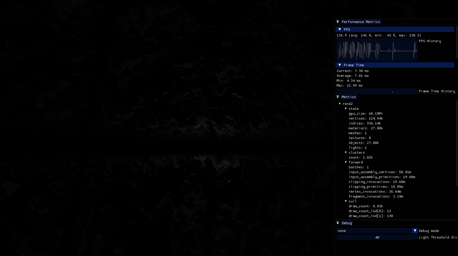![<RawText children='27000 dragons, 10000 lights.'>](https://logdahl.net/i/gpu-driven/drgs1.png)27000 dragons, 10000 lights。![<RawText children='A single light with a 1/40 influence range. Apologies for the dark image.'>](https://logdahl.net/i/gpu-driven/drgs2.png)一个范围为 1/40 的单灯。 抱歉图像黑暗。
# 未点亮
这就是我今天要分享的全部内容。 我希望这可以帮助激发你关于并行化的一些想法！ 如果你发现任何问题，或者你对如何超越它有想法，请随时给我发送电子邮件 (olle at logdahl dot net)！ ;)
- 30 -
# 下一步阅读